Dynamic Swarm Navigation

This project was undertaken as part of Inter-IIT Tech Meet 13.0 at IIT Bombay, based on a problem statement provided by Kalyani Bharatforge. Titled “Centralized Intelligence for Dynamic Swarm Navigation,” the project aimed to develop an effective approach for swarm navigation in continuously evolving environments.

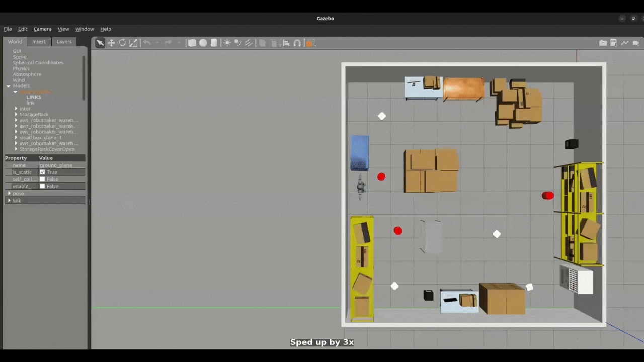
Figure 1: Small Swarm Navigation

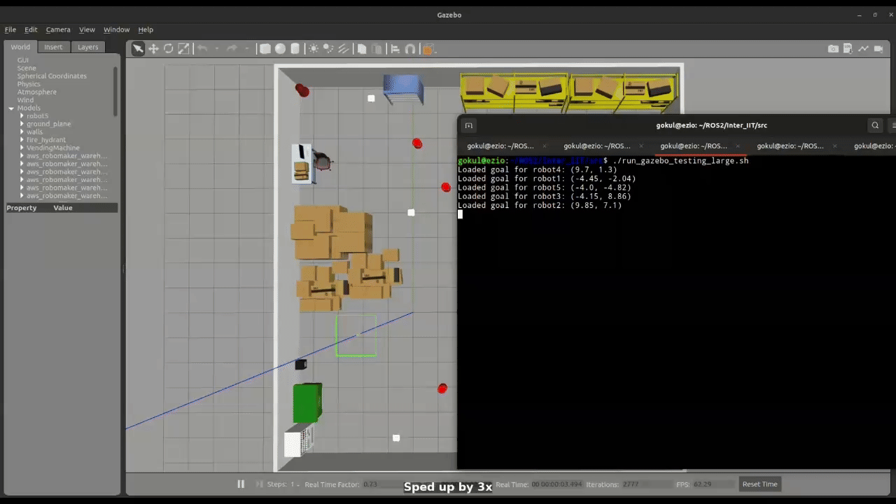
Figure 2: Large Swarm Navigation

Introduction

One of the essential technologies for creating smart robot swarms is motion planning. Traditional path planning methods in robotics require precise localization and complete maps, limiting their adaptability in dynamic environments. Reinforcement learning (RL), especially deep reinforcement learning (DRL), has emerged as a key strategy to address such issues.

Simulation

The simulation framework is developed in Gazebo Classic and integrated with ROS 2 Humble. Each robot carries a 2D LiDAR sensor used for obstacle detection. Robots are deployed at random positions in the environment, and their initial configurations are defined in a YAML file.

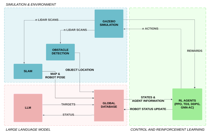
Figure 3: Illustration of Process Flowchart

Reinforcement Learning

The navigation task is formulated as a Markov Decision Process (MDP) represented by the tuple (S, A, S′, P, R), where each element holds its standard interpretation.

State Space

• Normalized Laser Scan Values: Measurements from the LiDAR, scaled to a normalized range.
• Normalized Goal Distance to Arena Size Ratio: The distance to the target goal, normalized relative to the size of the navigation area.
• Normalized Goal Heading Angle: The angle between the agent’s orientation and the direction to the goal, scaled to a normalized range.
• Previous Linear Velocity: The linear velocity of the agent during the prior time step.
• Previous Angular Velocity: The angular velocity of the agent during the prior time step.

Action Space

• Linear velocity: Bounded between [-1, 1]
• Angular velocity: Bounded between [-2, 2]

Reward Function

• Goal Alignment Penalty: A penalty applied for deviations in the heading angle from the optimal trajectory toward the goal.
• Excessive Angular Velocity Penalty: Penalizes the agent for executing abrupt or excessively large angular velocity actions.
• Proximity-to-Goal Reward: A reward inversely proportional to the Euclidean distance from the agent to the goal, encouraging progress toward the target.
• Obstacle Proximity Penalty: A penalty incurred when the agent approaches obstacles, discouraging unsafe trajectories.
• Excessive Linear Velocity Penalty: Penalizes the agent for employing large linear velocities that may compromise safety or stability.

RL Algorithm

The primary RL navigation framework is implemented using the Twin Delayed Deep Deterministic Policy Gradient (TD3) algorithm. TD3 is an advanced off-policy RL algorithm. The key reasons for selecting TD3 over alternative baseline algorithms are

• DDPG revealed a significant overestimation of Q-values, ultimately leading to policy degradation.
• PPO is computationally intensive and sample inefficient as compared to off-policy algorithms for large-scale navigation tasks.
• SAC and TD3 have the best data efficiency. However, SAC trains a stochastic policy, which does not guarantee convergence to a single optimal solution.

Methodology

The task was implemented as Decentralized Training and Decentralized Execution (DTDE). Initially, a single agent (robot) is trained within a dynamic environment. The trained networks are then deployed across multiple instances, corresponding to the number of robots.

Experiment and Simulation Results

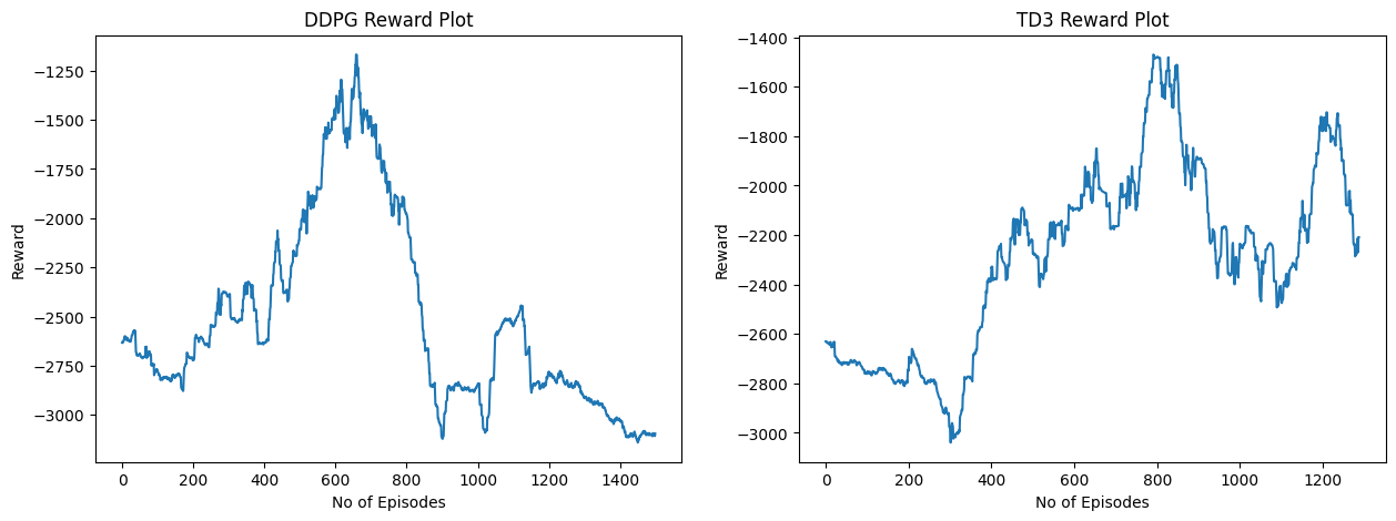
Figure 4: DDPG v/s TD3 Reward Plot

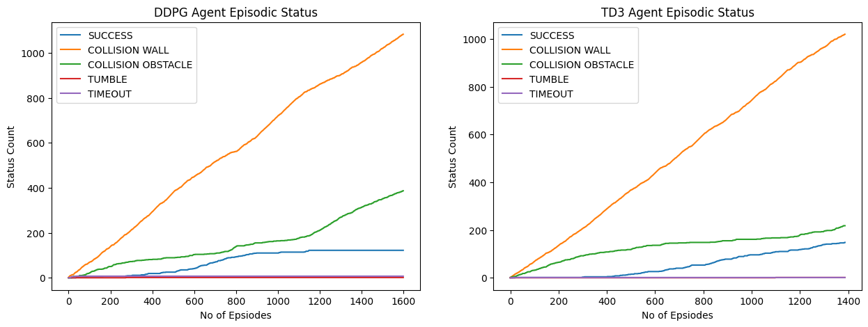
Figure 5: DDPG v/s TD3 Episodic Status Plot

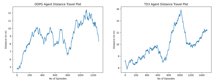
Figure 6: DDPG v/s TD3 Robot Distance Travel Plot