
Into the Diffusion World Part 1: DDPMs
This is a detailed blog on Denoising Diffusion Probabilistic Models. The objective is to present a comprehensive theoretical and mathematical background on DDPMs.
Why Diffusion ??
In recent times, the term “Diffusion” has gained significant attention in AI and Robotics research. For example, the paper Diffusion Policy leverages diffusion models to learn multimodal action distributions, enabling the generation of complex robotic behaviors. Similarly, the paper Policy Representation via Diffusion Probability Model for RL explores the use of diffusion models for online model-free reinforcement learning tasks.
This growing interest led me to delve deeper into Denoising Diffusion Probabilistic Models (DDPMs). In this blog, I will provide a comprehensive theoretical and mathematical background on DDPMs.
What are Diffusion Models ??
Diffusion models are a family of probabilistic generative models that progressively destroy data by injecting noise and then learn to reverse this process for sample generation.
Denoising Diffusion Probabilistic Models (DDPM)
DDPMs uses 2 markov chains,
- Forward diffusion process: slowly injects noise to the data
- Reverse diffusion process: slowly converts noise back to data.
It can also be viewed as a generative model consisting of an encoder and a decoder. The encoder takes a data sample and maps it through a series of intermediate latent variables. The decoder reverses this process. The mappings in both the encoder and decoder are stochastic rather than deterministic.
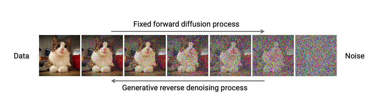
Figure 1: DDPM Forward and Reverse Markov Chains
Forward Diffusion Process
The goal of the forward process is to transform the given data distribution into a simple prior distribution. The paper assumes the simple prior to be a Standard Gaussian \( \mathcal{N}(0, I) \).
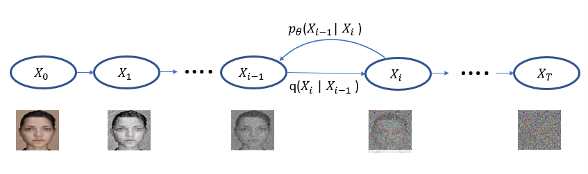
Figure 1: DDPM Forward Chain. Injecting noise till it becomes a pure standard gaussian noise
Given a data distribution \(x_{0} \sim q(x_{0}) \), the forward chain generates a sequence of random variables \( x_{1}, x_{2}, \dots x_{T} \) using a transition kernel \( q(x_{t} \mid x_{t-1})\). The joint distribution conditioned on \(x_{0}\) can be written as
\[ q(x_{1}, \dots, x_{T} \mid x_{0}) = \prod_{t=1}^{T} q(x_{t} \mid x_{t-1}) \]
So now we have to design a transitional kernel to incrementally tranform \(q(x_{0})\) to a tractable prior distribution. One common design choice is Gaussian perturbation.
\[ q(x_{t} \mid x_{t-1}) = \mathcal{N}(x_{t}; \sqrt{1-\beta_{t}} \, x_{t-1}, \beta_{t} I) \]
where \(\beta_{t} \in (0,1)\) is a hyperparameter. It determines how quickly the noise is blended and are collectively known as noise schedule. One of the reason to choose gaussian perturbation is that, it allows us to obtain the analytical form of \(q(x_{t} \mid {x_{0}})\) for all \(t \in (0, 1, \dots, T)\). Lets see the math.
We can use the reparameterization trick to sample a point \(x_{t}\). Let’s assume \(\alpha_{t} = 1-\beta_{t}\)
\[ x_{t} = \sqrt{1 - \beta_{t}} \, x_{t-1} + \sqrt{\beta_{t}} \, \epsilon_{t-1} \]
\[ x_{t} = \sqrt{\alpha_{t}} \, x_{t-1} + \sqrt{1 - \alpha_{t}} \, \epsilon_{t-1} \] where \(\epsilon_{t-1}, \epsilon_{t-2}, \dots \sim \mathcal{N}(0, I)\), so i am dropping the time dependance for now. Similarly we can write for timestep (t-1) and substitute. \[ x_{t-1} = \sqrt{\alpha_{t-1}} \, x_{t-2} + \sqrt{1 - \alpha_{t-1}} \, \epsilon \]
\[ x_{t} = \sqrt{\alpha_{t}} (\sqrt{\alpha_{t-1}} \, x_{t-2} + \sqrt{1 - \alpha_{t-1}} \, \epsilon) + \sqrt{1 - \alpha_{t}} \, \epsilon \]
\[ x_{t} = \sqrt{\alpha_{t}. \alpha_{t-1}} \, x_{t-2} + \sqrt{\alpha_{t}(1 - \alpha_{t-1})} \, \epsilon + \sqrt{1 - \alpha_{t}} \, \epsilon \]
Let’s do it another time to understand the pattern,
\[ x_{t} = \sqrt{\alpha_{t}. \alpha_{t-1}. \alpha_{t-2}} \, x_{t-3} + \sqrt{\alpha_{t}. \alpha_{t-1}(1 - \alpha_{t-2})} \, \epsilon + \sqrt{\alpha_{t}(1 - \alpha_{t-1})} \, \epsilon + \sqrt{1 - \alpha_{t}} \, \epsilon \]
Except the first term, all other terms are Gaussians with 0 mean, so their variances add up,
\[ x_{t} = \sqrt{\alpha_{t}. \alpha_{t-1}. \alpha_{t-2}} \, x_{t-3} + \sqrt{\cancel{\alpha_{t}. \alpha_{t-1}} - \alpha_{t}. \alpha_{t-1}. \alpha_{t-2} + \cancel{\alpha_{t}} - \cancel{\alpha_{t}. \alpha_{t-1}} + 1 - \cancel{\alpha_{t}}} \, \epsilon \]
\[ x_{t} = \sqrt{\alpha_{t}. \alpha_{t-1}. \alpha_{t-2}} \, x_{t-3} + \sqrt{1 - \alpha_{t}. \alpha_{t-1}. \alpha_{t-2}} \, \epsilon \]
Ok, I see a pattern here, lets write the general equation \[ x_{t} = \sqrt{\alpha_{t}. \alpha_{t-1}. \alpha_{t-2}. \dots \alpha_{0}} \, x_{0} + \sqrt{1 - \alpha_{t}. \alpha_{t-1}. \alpha_{t-2}. \dots \alpha_{0}} \, \epsilon \] \[ \boxed{x_{t} = \sqrt{\bar{\alpha_{t}}} \, x_{0} + \sqrt{1 - \bar{\alpha_{t}}} \, \epsilon} \]
Now, this equation is of greater importance as it gives \(x_{t}\) directly from \(x_{0}\), with just the need to compute \(\bar{\alpha_{t}} = \prod_{i=1}^{T} \alpha_{i}\). We’ll save this equation for later.
Importance of hyperparameter \( \beta_{t} \)
\(\beta_{t}\) controls the amount of gaussian noise added. It is chosen to be very small. It ensures that the noise is added gradually to the data over many steps. This choice is crucial because it preserves the structure of data for longer, making it easier for reverse process to reconstruct better images. The authors use a linear schedule over 1000 steps from \(\beta_{1} = 0.0001\) to \(\beta_{T} = 0.02\).
Reverse Diffusion Process
The goal of the reverse process is to sample a noise from the gaussian noise distribution and remove noise gradually in the reverse time direction to get clean images.
From the above sentence, all I can understand mathematically is to figure out the transition kernel \(q(x_{t-1} \mid x_{t})\). Seems easy, but we can’t estimate this, because it will require the entire dataset. So we’ll learn an approximation to this estimate using neural networks \(p_{\theta}(x_{t-1} \mid x_{t})\).
\[ p_{\theta}(x_{t-1} \mid x_{t}) = \mathcal{N}(x_{t-1}, \mu_{\theta}(x_{t}, t), \sum_{\theta}(x_{t}, t)) \]
Objective
Like in VAE, we would like to maximize the log-likelihood of the observed data \(p_{x_{0}}\) which can be written the sum of joint distributions.
\[ \log p_{x_{0}} = \log \int p(x_{0:T}) dx_{1:T} \] \[ \log p_{x_{0}} = \log \int p(x_{0:T}) \frac{q(x_{1:T} \mid x_{0})}{q(x_{1:T} \mid x_{0})} dx_{1:T} \] \[ \log p_{x_{0}} = \log \mathbb{E_{q(x_{1:T} \mid x_{0})}} [ \frac{p(x_{0:T})}{q(x_{1:T} \mid x_{0})}] \] \[ \log p_{x_{0}} \geq \mathbb{E_{q(x_{1:T} \mid x_{0})}} [ \log \frac{p(x_{0:T})}{q(x_{1:T} \mid x_{0})}] \]
Ok, so now we will study the term inside log in the right side.
\[ \log \frac{p(x_{0:T})}{q(x_{1:T} \mid x_{0})} = \log \frac{p(x_{T}) \prod_{t=1}^{T} p_{\theta}(x_{t-1} \mid x_{t})}{q(x_{1} \mid x_{0}) \prod_{t=2}^{T} q(x_{t} \mid x_{t-1}, x_{0})} \]
Let’s analyse the denominator, and use Bayes Rule
\[ q(x_{1} \mid x_{0}) \prod_{t=2}^{T} q(x_{t} \mid x_{t-1}, x_{0}) = q(x_{1} \mid x_{0}) \prod_{t=2}^{T} \frac{q(x_{t-1} \mid x_{t}, x_{0}) q(x_{t} \mid x_{0})}{q(x_{t-1} \mid x_{0})} \]
This after expanding the product simplifies to the following
\[ q(x_{1} \mid x_{0}) \prod_{t=2}^{T} q(x_{t} \mid x_{t-1}, x_{0}) = q(x_{T} \mid x_{0}) \prod_{t=2}^{T} q(x_{t-1} \mid x_{t}, x_{0}) \]
Great, we’ll put this back into the equation and do more simplification
\[ \log \frac{p(x_{0:T})}{q(x_{1:T} \mid x_{0})} = \log \frac{p(x_{T}) \prod_{t=1}^{T} p_{\theta}(x_{t-1} \mid x_{t})}{q(x_{T} \mid x_{0}) \prod_{t=2}^{T} q(x_{t-1} \mid x_{t}, x_{0})} \]
\[ \log \frac{p(x_{0:T})}{q(x_{1:T} \mid x_{0})} = \log \frac{p(x_{T}) p_{\theta}(x_{0} \mid x_{1}) \prod_{t=2}^{T} p_{\theta}(x_{t-1} \mid x_{t})}{q(x_{T} \mid x_{0}) \prod_{t=2}^{T} q(x_{t-1} \mid x_{t}, x_{0})} \]
Now let’s breakdown the log equation to 3 terms
\[ \log \frac{p(x_{0:T})}{q(x_{1:T} \mid x_{0})} = \log \frac{p(x_{T})}{q(x_{T} \mid x_{0})} + \log p_{\theta}(x_{0} \mid x_{1}) + \sum_{t=2}^{T} \log \frac{p_{\theta}(x_{t-1} \mid x_{t})}{q(x_{t-1} \mid x_{t}, x_{0})} \]
\[ \log p_{x_{0}} \geq \mathbb{E_{q(x_{1:T} \mid x_{0})}} [ \log \frac{p(x_{T})}{q(x_{T} \mid x_{0})} + \log p_{\theta}(x_{0} \mid x_{1}) + \sum_{t=2}^{T} \log \frac{p_{\theta}(x_{t-1} \mid x_{t})}{q(x_{t-1} \mid x_{t}, x_{0})} ] \]
Nice, from the 3 terms, first term can be removed as it has no dependance on \(\theta\). The last term is interesting. It looks like a bunch of KL divergences summed up. The denominator is the estimate for reverse process and the numerator is the approximation. So all we need to do is to minimize the distributional distance. But wait, roadblock, we don’t know \(q(x_{t-1} \mid x_{t}, x_{0})\). Hmmm, Let’s try bayes rule.
\[ q(x_{t-1} \mid x_{t}, x_{0}) = \frac{q(x_{t} \mid x_{t-1}, x_{0}) \, q(x_{t-1} \mid x_{0})}{q(x_{t} \mid x_{0})} \]
Ok, each term in the right is a gaussian, let’s maybe use the exponential form, which may help simplify stuffs.