This is a detailed blog on Dynamic Programming, a collection of algorithms to compute optimal policies in Reinforcement Learning. This post will cover the detailed math concepts.

Introduction

Dynamic Programming (DP) is a collection of algorithms used to compute optimal policies given a perfect model of the environment as a MDP. DP can be used to find exact solutions in some finite cases. For continous problems, the states and actions are discretized first, then DP is applied.

Classical DP methods are rarely used in RL today because of two shortcomings

• Assumption of perfect environment model
• Great Computational expense

But DP provides a foundation to study other methods. In fact, the other methods try to mimic the effect of DP, while reducing the computation or while working with approximate models.

Bellman Optimality Equations

We can find optimal policies once we have found the optimal state-value function \(v_{*}\) or state-action value function \(q_{*}\), which satisfy the Bellman optimality equation.

\[ V^{*}(s) = \max_{a} \ \mathbb{E} \left[ R_{t+1} + \gamma V^{*}(S_{t+1}) \mid S_{t}=s, A_{t}=a \right] \] \[ Q^{*}(s, a) = \mathbb{E} \left[ R_{t+1} + \gamma \max_{a^{‘}}Q^{*}(S_{t+1}, a^{‘}) \mid S_{t}=s, A_{t}=a \right] \]

Policy Evaluation (Prediction Problem)

Policy evaluation computes the state-value function \(v_{\pi}\) for an arbitrary policy \(\pi\)

From the definition of state-value function, which is the expected return \[ v_{\pi}(s) = E_{\pi} [G_{t} \mid S_{t} = s] \] \[ v_{\pi}(s) = E_{\pi} [R_{t+1} + \gamma G_{t+1} \mid S_{t} = s] \] \[ v_{\pi}(s) = E_{\pi} [R_{t+1} + \gamma v_{\pi}(S_{t+1}) \mid S_{t} = s] \] \[ \boxed{ v_{\pi}(s) = \sum_{a} \pi(a \mid s) \sum_{s^{‘}, r} \ p(s^{‘}, r \mid s, a) \left[r + \gamma v_{\pi}(s^{‘}) \right]} \]

The existence and uniqueness of \(v_{\pi}\) is guaranteed as long as either \(\gamma < 1\) or eventual terminaton is guaranteed from all states under policy \(\pi\)

If we know the complete environment dynamics, then the above equation is a system of \(len(S)\) simultaneous linear equations with \(len(S)\) unknowns, which is straightforward to solve, but tedious. So we use iterative method to solve the equation. We initialize the value function arbitrarily and use the above equation as update rule to get new approximation. The sequence of approximations \((v_{k})\) converges to \(v_{\pi}\) as \(k \to \infty\). This algorithm is called iterative policy evaluation.

Iterative policy evaluation converges only in the limit, but in practice we use a small threshold to stop the updates. Given below is the pseudocode of the algorithm.

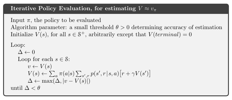
Figure 1: Iterative Policy Evaluation Algorithm (Source: Sutton & Barto)